Deep learning (DL) is rapidly becoming one of the most prominent topics in the realm of materials data science, with a quickly expanding array of applications across many functions. It can also refer to a method that sees things as separate units rather than a whole, image-based, spectral, and textual data types. DL facilitates the examination of unstructured data and the automated recognition of neural connections, such as in a consumer’s buying decisions.
The recent creation of extensive materials databases has particularly propelled the use of DL techniques in atomistic predictions. Conversely, progress in image and spectral data has primarily utilised synthetic data generated by high-quality forward models and generative unsupervised DL methods.
For each data type, we explore applications that include both theoretical and experimental data, common modeling strategies along with their advantages and drawbacks, as well as pertinent publicly accessible software and datasets. We wrap up the review by discussing recent interdisciplinary work focused on uncertainty quantification in this area and offer a brief outlook on limitations, challenges, and possible growth opportunities for DL techniques within materials science. “Processing-structure-property-performance” is a central principle in Materials Science and Engineering (MSE).
The scales in length and time associated with material structures and phenomena differ considerably among these four components, adding additional complexity. For example, structural data can range from precise atomic coordinates of elements to the microscale distribution of phases (microstructure), to connectivity of fragments (mesoscale), and images and spectra. Drawing connections between these components presents a significant challenge. Both experimental and computational methods are valuable in uncovering such relationships between product purchase selection. With the rapid advancement in the automation of experimental instruments and the massive growth in computational capabilities, the volume of public materials datasets has surged exponentially.
Numerous large experimental and computational datasets have emerged through the Materials Genome Initiative (MGI) and the increasing embrace of Findable, Accessible, Interoperable, Reusable (FAIR) principles. This surge of data necessitates automated analysis, which can be facilitated by machine learning (ML) approaches.
DL applications are swiftly replacing traditional systems in various facets of everyday life, such as image and speech recognition, online searches, fraud detection, email/spam filtering, and financial risk assessment, among others. DL techniques have demonstrated their ability to introduce exciting new functionalities across numerous domains (including playing Go, autonomous vehicles, navigation, chip design, particle physics, protein science, drug discovery, astrophysics, object recognition, and more). Recently, DL methods have begun to surpass other machine learning approaches in multiple scientific disciplines, including chemistry, physics, biology, and materials science.
The application of DL in MSE remains relatively novel, and the field has yet to fully realise its potential, implications, and limitations. DL offers innovative methods for exploring material phenomena and has encouraged materials scientists to broaden their conventional toolkit. DL techniques have proven to serve as a complementary strategy to physics-based methods in materials design. Although large datasets are often regarded as essential for successful DL applications, strategies such as transfer learning, multi-fidelity modeling, and active learning can frequently render DL applicable for smaller datasets as well.
General machine learning concepts
Although deep learning (DL) techniques offer numerous benefits, they also come with drawbacks, the most prominent being their opaque nature, which can obstruct our understanding of the physical processes being studied. Enhancing the interpretability and explainability of DL models continues to be a vibrant area of investigation.
Typically, a DL model comprises thousands to millions of parameters, complicating the interpretation of the model and the direct extraction of scientific insights. While there have been several commendable recent reviews on machine learning (ML) applications, the rapid progress of DL in materials science and engineering (MSE) necessitates a focused review to address the surge of research in this area
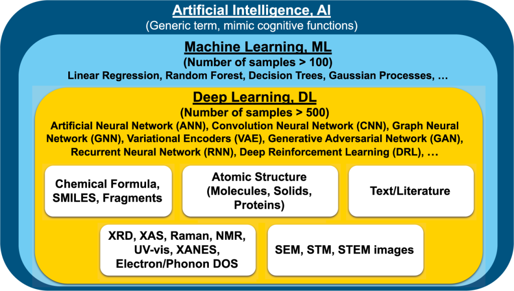
Artificial intelligence (AI) refers to the creation of machines and algorithms that replicate human intelligence, for example, by optimising actions to achieve specific objectives. Machine learning (ML) is a branch of AI that enables systems to learn from data without being explicitly programmed for a particular dataset, such as in chess playing or social network recommendations. Deep learning (DL) is a further subset of ML that draws inspiration from biological brains and employs multilayer neural networks to tackle ML tasks.
Commonly used ML techniques include linear regression, decision trees, and random forests, where generalised models are trained to determine coefficients, weights, or parameters for a specific dataset. When applying traditional ML methods to unstructured data (like pixels or features from images, sounds, text, and graphs), challenges arise because users must first extract generalised, meaningful representations or features on their own (for instance, calculating the pair distribution for an atomic structure) before training the ML models. This makes the process labor-intensive, fragile, and difficult to scale.
This is where deep learning (DL) techniques gain significance. DL methods rely on artificial neural networks and related techniques. According to the “universal approximation theorem,” neural networks can approximate any function with arbitrary precision. However, it is crucial to recognise that this theorem does not ensure that these functions can be learned effortlessly.
Neural networks
Perceptron A, also known as a single artificial neuron, serves as the fundamental unit of artificial neural networks (ANNs) and facilitates the forward transmission of information. For a collection of inputs [x1, x2, …, xm] directed towards the perceptron, we assign real-valued weights (and biases to adjust these weights) [w1, w2, …, wm], which we then multiply together correspondingly to produce a cumulative sum.
Some widely used software frameworks for training neural networks include PyTorch, TensorFlow, and MXNet. It is important to acknowledge that certain commercial devices, instruments, or materials are referenced in this document to clarify the experimental methodology. This mention is not meant to suggest any endorsement or recommendation by NIST, nor does it imply that the identified materials or equipment are definitively the best options available for the intended purpose.
Activation function: Activation functions (including sigmoid, hyperbolic tangent [tanh], rectified linear unit (ReLU), leaky ReLU, and Swish) are essential nonlinear elements that allow neural networks to combine numerous simple components to learn intricate nonlinear functions. For instance, the sigmoid activation function transforms real numbers to the interval (0, 1); this function is frequently utilised in the final layer of binary classifiers to represent probabilities.
The selection of an activation function can influence both the efficiency of training and the ultimate accuracy. Loss function, gradient descent, and normalization The weight matrices of a neural network are either initialised randomly or derived from a pre-trained model. These weight matrices interact with the input matrix (or the output from a previous layer) and are processed through a nonlinear activation function to generate updated representations, commonly referred to as activations or feature maps. The loss function (sometimes called the objective function or empirical risk) is computed by comparing the neural network’s output with the known target value data.
Typically, the weights of the network are iteratively adjusted using stochastic gradient descent algorithms to reduce the loss function until the desired level of accuracy is reached. Most contemporary deep learning frameworks support this process by employing reverse-mode automatic differentiation to calculate the partial derivatives of the loss function about each network parameter through the continuous application of the chain rule. This process is informally known as back-propagation. Common algorithms for gradient descent include Stochastic Gradient Descent (SGD), Adam, and Adagrad, among others.
The learning rate is a crucial parameter in gradient descent. Except SGD, all other methods utilise adaptive tuning for learning parameters. Depending on the specific goal, whether classification or regression, various loss functions, such as Binary Cross Entropy (BCE), Negative Log Likelihood (NLL), or Mean Squared Error (MSE) are employed. Typically, the inputs of a neural network are scaled, meaning they are normalised to achieve a zero mean and a unit standard deviation. Scaling is also applied to the inputs of hidden layers (through batch or layer normalisation) to enhance the stability of artificial neural networks.
Convolutional neural networks
Convolutional neural networks (CNNs) can be understood as a refined version of multilayer perceptrons that carry a significant inductive bias towards learning image representations that are invariant to translation. There are four primary elements in CNNs: (a) learnable convolutional filter banks, (b) nonlinear activation functions, (c) spatial downsampling (achieved through pooling or strided convolution), and (d) a prediction component, which typically includes fully connected layers that process a global representation of the instance.
In CNNs, we utilize convolution operations with multiple kernels or filters that possess trainable and shared weights or parameters, rather than standard matrix multiplication. These filters or kernels are matrices with a relatively small number of rows and columns that convolve across the input to automatically extract high-level local features represented as feature maps.
The filters slide (perform element-wise multiplication) across the input using a fixed number of strides to generate the feature map, and the information acquired is then passed to the hidden or fully connected layers. Depending on the nature of the input data, these filters may be one, two, or three-dimensional. As with fully connected neural networks, nonlinearities like ReLU are subsequently applied, enabling us to handle complex and nonlinear data.
The pooling operation maintains spatial invariance while downsampling and reducing the dimensionality of each feature map created post-convolution. These downsampling or pooling processes can take various forms, such as max pooling, min pooling, average pooling, and sum pooling. After one or more layers of convolution and pooling, the outputs are typically condensed into a one-dimensional global representation. CNNs are particularly favoured for image data.
Graph neural networks
Traditional CNNs, as previously mentioned, rely on regular grid Euclidean data (like 2D grids found in images). However, real-world data structures, including social networks, image segments, word embeddings, recommendation systems, and atomic/molecular formations, are typically non-Euclidean.
In these instances, graph-based non-Euclidean data structures become particularly significant. From a mathematical standpoint, a graph G is characterized as a collection of nodes/vertices V, a collection of edges/links E, and node attributes/features X: G = (V, E, X). This framework can effectively represent non-Euclidean data. An edge connects a pair of nodes and conveys the relational information between them. Each node and edge may possess specific attributes/features.
An adjacency matrix A is a square matrix that signifies whether nodes are connected, represented by 1 (connected) or 0 (not connected). Graphs can be categorized into various types, including undirected/directed, weighted/unweighted, homogeneous/heterogeneous, and static/dynamic. An undirected graph reflects symmetric relationships between nodes, whereas a directed graph showcases asymmetric relationships such that Aij ≠ Aji.
In a weighted graph, each edge is assigned a scalar weight instead of merely 1s and 0s. A homogeneous graph consists of nodes that all represent instances of the same type, with edges that capture relationships of the same kind, while a heterogeneous graph can include nodes and edges of different types. Heterogeneous graphs facilitate the management of diverse node and edge types along with their associated features.
When input features or graph structures change over time, they are classified as dynamic graphs; otherwise, they are regarded as static. If a node connects to another node multiple times, it is referred to as a multi-graph. Categories of GNNs Currently, GNNs are likely the most favoured AI approach for predicting various material properties based on structural data. Graph neural networks (GNNs) are deep learning techniques that function within the graph domain and can capture graph dependencies through message passing among nodes and edges.
GNN training involves two primary steps: (a) initially aggregating data from neighbouring nodes and (b) updating the nodes and/or edges. Notably, the aggregation process is invariant to permutations. Similar to fully connected neural networks, the input node features, X (along with the embedding matrix), are multiplied by the adjacency matrix and weight matrices, followed by the application of a nonlinear activation function to yield outputs for the subsequent layer.
This process is known as the propagation rule. Depending on the propagation rule and aggregation techniques, various types of GNNs can exist, including Graph Convolutional Networks (GCN), Graph Attention Networks (GAT), Relational-GCN, Graph Recurrent Networks (GRN), Graph Isomorphism Networks (GIN), and Line Graph Neural Networks (LGNN). Among these, Graph Convolutional Networks are the most widely used GNNs.
Sequence-to-sequence models
Historically, learning from sequential data like text has involved creating a fixed-length input derived from the information. For instance, the “bag-of-words” method merely counts how many times each word appears in a document, resulting in a fixed-length vector that corresponds to the total vocabulary size. On the other hand, sequence-to-sequence models can take into account the sequential or contextual nuances of each word, producing outputs of varying lengths.
For example, in named entity recognition (NER), a sequence of words (such as a chemical abstract) is transformed into an output sequence of “entities” or classifications, where each word is designated a specific category. An early iteration of the sequence-to-sequence model is the recurrent neural network, or RNN. Unlike the fully connected neural network architecture, which lacks connections between hidden nodes on the same layer and only connects nodes across adjacent layers, RNNs incorporate feedback connections.
Each hidden layer can be expanded and processed like conventional neural networks that share the same weight matrices. There are several variants of RNNs, with the most prevalent being gated recurrent unit recurrent neural network (GRURNN), long short-term memory (LSTM) network, and clockwork RNN (CW-RNN). Nonetheless, all these RNN types face certain limitations, including (i) challenges with parallelisation, leading to difficulties in training on extensive datasets, and (ii) issues with maintaining long-range contextual information due to the “vanishing gradient” phenomenon.
However, as we will discuss later, LSTMs have been effectively utilized in various NER challenges within the materials sector. More recently, sequence-to-sequence models built on a “transformer” architecture, such as Google’s Bidirectional Encoder Representations from Transformers (BERT) model, have begun to tackle some of the problems associated with traditional RNNs. Instead of passing a state vector that processes each word sequentially, these models implement an attention mechanism, which enables simultaneous access to all previous words without relying on specific time steps. This approach enhances parallelisation and improves the retention of long-term context.