


Our purpose in this article is to provide a point of empirical evidence as to how machine-learning techniques stack up in their ability to predict consumer choices, relative to traditional statistical techniques. We compare a traditional (naïve) multinomial logit to six machine-learning alternatives: Learning Multinomial Logit, Random Forests, Neural Networks, Gradient Boosting, Support Vector Machines and an Ensemble Learning Algorithm.
Definition of Logit
The logit function is mathematically defined as the logarithm of the odds of the probability p of a certain event occurring: Logit(p) = log(p / (1 – p)) Here, p represents the probability of the event, and log denotes the natural logarithm.
The comparison is done by applying these methods to stock-keeping unit (SKU) level panel data. Results show that machine-learning techniques tend to perform better, but not always. Ensemble learning performs best while maintaining an overall high-performance level across all SKU classes, independently of their sample size.
This result builds on existing evidence about the benefits of combining multiple prediction techniques over-relying on a single best-performing model, as conventional wisdom would intuitively make us believe. In general, the better performance of machine learning techniques at predicting product choice should not come as a surprise. At their core, machine learning techniques are designed to augment the dimensionality of models and/or scan through orders of magnitude greater model alternatives, relative to the narrower focus of traditional approaches.
Introduction
Machine-learning techniques have been gaining ground over traditional statistics in most fields, particularly among practitioners. Social sciences including marketing and economics are no exception. However, the quantitative foundations of these two fields have historically been rooted in interpretability and causal inference, while machine learning is generally understood to be stronger at predicting but relatively weaker at interpretability and hypothesis testing.
The contribution here is to provide a point of comparison across a wide set of machine-learning techniques in their ability to predict consumer choices relative to more traditional statistical techniques and uncover their performance strengths and weaknesses in the context of a typical consumer product choice problem.
The greatest conceptual difference between traditional statistical techniques and machine learning is that in the former a hypothesis is proposed in the form of a stylised mathematical model that is then tested; while the latter allows for greater mathematical construct flexibility, without explicit regard for theoretical foundations, as it tries to maximise predictive accuracy.
One can also argue that from a procedural standpoint, five relatively common elements of machine learning distinguish it from traditional statistics in their systematic application:
(1) data preprocessing
(2) feature engineering
(3) data splitting between training and test sets
(4) cross-validation
(5) use of tuning parameters (Kuhn and Johnson 2013).
This is not to say that traditional statistics has not applied any of these steps, generally speaking; but perhaps, that they have been less central and widespread in their application.
Data preprocessing tends to focus on, among other transformations, the centring and scaling of predictor features by subtracting their mean and dividing them by their dispersion statistic, often the standard deviation. Removal of skewness is also often applied to the data by replacing raw input feature values with log, square root, inverse, or Box-Cox transformations.
The treatment of missing values is also confronted head-on with imputation techniques that quite often lean on other predictive machine learning techniques, like k-nearest-neighbours. One of the main reasons behind these manipulations of the raw data is to contribute to the smoothness, speed, and numerical stability of the high computational demands associated with machine-learning parameter estimation.
Feature engineering is also not unique to machine learning, but ubiquitous relative to traditional statistics. Techniques like principal components or factor analysis have been commonplace in applied statistics as ways to reduce the dimensionality of models, resulting in among other benefits lower Multicollinearity and Overfitting.
However, machine learning has taken this further with its foundational reliance on non-linear transformations like polynomials, hinge functions and kernels. These approaches often seek not to reduce dimensionality, but rather grow it (sometimes in ways that generate negative degrees of freedom) to capture nuances that improve a model’s predictive performance. Often, multiple versions of engineered features are tested in the model iteratively, leveraging cross-validation (discussed below).
Splitting the data into training and test sets relies on random (and in some cases stratified, to maintain a proportional distribution of feature values) sampling of the original data set. Its intent is primarily to evaluate a model on data it has not seen before, as a true gauge of a model’s predictive ability. One can understand that this is important to machine learning since its application is heavily oriented towards actionable prediction, particularly amongst practitioners. In traditional statistics or econometrics, models are often evaluated on the full dataset, and less frequently on an out-of-sample set aside from the full dataset.
Cross-validation is perhaps one of the most salient departures of machine-learning techniques. The training dataset itself is split into multiple training subsets. This is, therefore, analogous to splitting the original full dataset into training and test sets. However, a key difference is its reliance on resampling techniques rooted in bootstrapping (Efron and Tibshirani 1993).
It involves randomly dividing the training set observations with resampling into two parts: a training subset and a validation set (more commonly, multiple validation sets). The model is fit on the training subset and the fitted model is then used to predict responses for the observations in the validation set. Resampling, refitting and evaluation of the model are done multiple times. Two common resampling techniques used for cross-validation are leave-one-out and k-fold.
A key benefit of cross-validation is the estimation of how sensitive a model is to small changes in input data. Cross-validation results are often summarised with the mean or some other form of aggregation of the multiple model performance scores. Another application of cross-validation is to compare the performance of multiple somewhat different versions of a model to select the best-performing one. This is related to the next key element of machine learning: tuning parameters.
Tuning parameters (also called hyperparameters) are fundamental to machine learning, and a significant departure relative to traditional statistics. Tuning parameters shape model and/or loss/objective functions to select model parameter values. They typically do not have analytical solutions and instead rely on numerical search algorithms. Thus, tuning parameters requires an iterative trial-and-error approach or numerical optimisation algorithm across a preselected number or range of values to evaluate. As described above, this is done through cross-validation. Cross-validation to find optimal tuning parameter values is executed as follows:
- Step 1: Identify several alternative models to run, based on tuning parameters to be tested.
- Step 2: For each model alternative
- Step 2.1: Split the training data into a training subset and one or several validation sets.
- Step 2.2: Fit the model to the training subset data.
- Step 2.3: Estimate the performance of the model against validation sets.
- Step 3: After all model alternatives have been run, aggregate, and contrast the results of all model alternatives.
- Step 4: Select the best-performing model, as shaped by a specific set of potential tuning parameters.
- Step 5: Re-fit the best-performing model on the entire training dataset to update model parameters.
The objective here is to determine whether machine learning models are superior to traditional statistical models at predicting consumer choice. More specifically it compares the SKU consumer choice predictive ability of a traditional (called naïve moving forward) multinomial logit model against six of its relatively more relevant machine-learning classification alternatives, in a realistic setting.
There are better sources for a comprehensive treatise of the approaches leveraged in this paper (Hastie et al. 2009). The data used for the analyses is grocery scanner panel data for category purchases from Information Resources, Inc.’s academic dataset (Bronnenberg et al. 2008). The metrics applied to determine the performance of the different models are Sensitivity, Accuracy and Cohen’s Kappa. These three-performance metrics are some of the most commonly used ones for classification problems, such as brand or product choice prediction.
Machine Learning for Product Choice: Data
This dataset is offered and maintained by the marketing research firm Information Resources (IRI) now called Circana, parent company Hellman & Friedman in Chicago the U.S. It is intended to enable academic researchers with the ability to study important topics in marketing and economics that are of concern to practitioners, policy-makers, and scholars. Well-recognised in the consumer-packaged goods space amongst academicians, it has broadly been applied to marketing research.
Twelve years of weekly store-level data for grocery chains and drug stores in 47 markets is provided. It also offers panel purchase and demographic data for two of IRI’s Behaviour Scan markets (11 years, for the same categories). While not used here, TNS advertising data for two categories for some early years are also applied.
For our purposes here, three full years of data are used. However, the first year is used to provide historical values used as predictors. Thus, for the modelling exercise, a third of the observations are lost to create lagged variables for observations. As a result, the modelling relies on 35,391 observations, with no missing values.
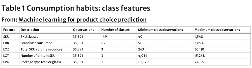
The dataset contains 149 category SKUs, ranging from 40 to 1,548 observations for each class value, and an average of 237.5. The dataset was constrained to only contain SKUs with at least 40 observations. SKUs are coded as SKU1-SKU149, rather than by product name. The models try to forecast a panelist’s next purchase, based on the number of predictors featured, including prior purchase choices. Predictor features include the last choice made in terms of brand, volume content, number of units in the package, and package type (Table 1). The advent of AI, now allows us to also include human personality data, how long a product is viewed, how many times, and the pattern of pre and post-purchase human behaviour (be it a conscious thought or otherwise) offering insights into the human element of the individual making those decisions.
These are all treated as class features, and their descriptive statistics are shown in Table 1. The last brand purchased has a total of 62 levels, with at least 51 observations each. Last volume. content purchased has three levels (96, 144 and 196 oz), with a minimum of 263 observations each. Last-package units purchased has also three levels (6, 20 and 35 units), with a minimum of 4,934 observations.
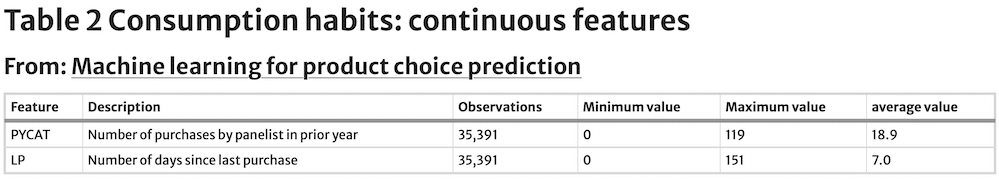
The last package type purchased has only two levels (can or glass). Table 2 contains two additional continuous predictor features: the number of category purchases made in the prior year and the number of days since the last purchase. The minimum value for the number of category purchases made in the prior year is zero days, the maximum is 119 days, and the average is 18.9 days. For the number of days since the last purchase, the minimum observed value is zero days, the maximum 151 and the average 7.0.
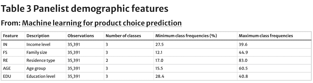
A third set of predictors featured are demographic characteristics of the panelists (Table 3). In the dataset, there are 3,404 unique panellists. The panelist observational frequencies range from one to 243 observations. The demographic features included are income, family size, residence type, age and education. All of them are treated as class features. For income, we have three levels: less than $35,000, $35,000 to $65,000 and more than $65,000.
The level with the smallest sample representation is more than $65,000 with a total of 27.5% of the observations. Family size has also three levels: one, two and greater than three. Of these three levels, the weakest representation is one, with 12.1% of the observations. The residence has two levels: owner and renter. The renters account for 17.0% of the observations in the dataset, while the rest are owners. Age has three levels: less than 45, between 45 and 54, and older than 54.
The class with the least representation in the dataset is less than 45 years old with 15.5% of the observations. Finally, education has also three levels: basic, high school, and at least some college. All are evenly distributed, with at least some colleges having the fewest observations (28.4%).
For all but the naïve multinomial logit model, data is preprocessed by centring and scaling each continuous feature. This is done as a way to free this benchmark model from one of the key systematic data treatments so commonly applied in machine learning, but less so in traditional modelling.
As mentioned before, there are many occasions when researchers and practitioners apply preprocessing to the data before running traditional multinomial models. Centering is achieved by subtracting the mean from each observation, while scaling relies on dividing each observation by the standard deviation of the feature values. The data is then randomly split into training (80%) and test (20%) datasets, while preserving the proportion of the product categories in the full dataset (thus, this is a stratified random split).
The 80/20 split while somewhat arbitrary is considered a good rule of thumb by Kuhn and Johnson (2013). Predictions on the test dataset are used as the ultimate arbiter of model performance. Except the naïve multinomial logit model (the baseline comparison or proxy for traditional statistics), training data is split again (this time with resampling) into a training and tenfold cross-validation dataset, following best practices (Kuhn and Johnson 2013). Estimation of feature and tuning parameters is based on tenfold cross-validation of the training dataset.
The cross-validation selects parameters that maximise the model with the greatest level of Accuracy (% of times the model predicts product choice observations accurately) against the training validation samples.
Models
The conceptual problem of predicting a consumer’s brand (that can be extended to SKU) choice can be framed in the form of a classification model (Russell 2014). Approaches supporting this type of model first predict the probability of each of the categories of a qualitative response feature, Yi, as the basis for making the classification. In its simplest form:
(1)
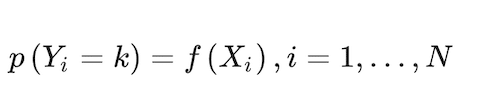
expresses the probability that the i-th choice falls in the k = 1,…,K kth category, where X is a set of predictor features, and i = 1,…,N is an index of all N observations in the dataset. In our case, Y {SKU1, …, SKU149}. X is composed of consumption habits, demographics, and marketing predictor features. Consumption habits include the last choices made for four class features: brand choice made, volume content, number of units in the package, and package type.
Consumption habits in X also include the number of category purchases made in the last year and the number of days since the last category purchase. Panelist demographic characteristics included in X are class features income, family size, residence, age and education. The last set of features included in X are store marketing conditions: whether the SKU is only featured in the retailer circular, only on a prominent display in the store, plus whether the SKU is on price reduction.
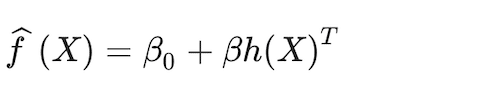
The function f(X) can take on various forms, depending on the approach selected. In addition, for the machine-learning approaches, the final model can include the full set, just a subset, or an augmented set of the initial X predictor elements through feature engineering. Further, X can be transformed linearly or non-linearly in various ways.
What follows is seven different ways of turning the conceptual abstraction of Eq. (1) into concrete model specifications and parameter estimations. The description of the approaches below focuses on defining the response model f(X) and the objective or loss function optimised to estimate model parameters, laying out the iterative processes to evaluate parameters and the tuning parameters involved.
Naïve Multinomial Logit
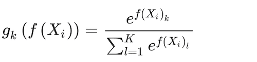
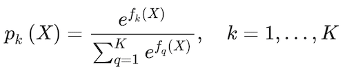
The Naïve Multinominal Logit Model is expressed as a log-linear functional form between the response and the predictor features, for ease of use (Venables and Ripley 2002). To make sure that the probabilities add up to one, f(X) is transformed by a softmax function (Bridle 1990):
(2)
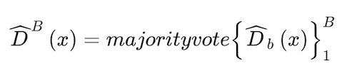
where and b = 1, …, B is the index for the number of random trees to estimate, B. In practice, each tree produces a class prediction for each observation D̂b(X). Then the final classification is solved by the majority vote across all b = 1, …, B trees
The parameters of this model are estimated by minimising the deviance function below:
(3)
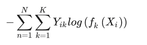
The corresponding classifier (that turns probabilities into classes) is G(x) = argmaxk fk(Xi)(Hastie et al. 2009). This is a loss function without regularisation, and therefore, without tuning parameters, of the type that is more commonplace in machine learning, rather than in traditional statistics (as this multinomial model is trying to represent). Parameters are estimated using maximum likelihood. Throughout the paper, we treat the performance of this model and its estimation procedure as the benchmark the rest of the models and their estimation approaches are compared against.
Learning Multinomial Logit
In this version of the model, the basic multinomial logit model leverages data preprocessing by scaling and centring it to improve estimation process smoothness. It also relies on regularisation to prevent overfitting by adding a decay tuning parameter (λ) to the deviance function in Eq. (3):
(4)
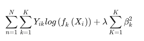
λ is the only tuning parameter in this algorithm that is estimated using standard tenfold cross-validation (Kuhn and Johnson 2013), thus incorporating an additional machine-learning element to the estimation. The parameters are estimated using maximum likelihood.
Random Forests
Random Forests (Breiman 2001) is a derivation of bagging, which in turn is a bootstrap version of the classification and regression tree (CART). Random forests’ advantage over bagging is that they rely on less correlated individual classification trees. Each time a split is considered, a random sample of mtry < rank(X) predictor features is selected as split candidates from the full set of predictors (James et al. 2013). We can express the random forest model as
(5)
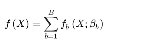
where and b = 1, …, B is the index for the number of random trees to estimate, B. In practice, each tree produces a class prediction for each observation. Then the final classification is solved by the majority vote across all b = 1, …, B trees
(6)
Each tree leverages a traditional classification tree approach, using the Gini criterion to guide the splitting by Breiman et al. (1984), as in
(7)
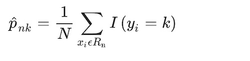
Where the proportion of class k observations in node n, and where I(yi = k) is an indicator conditional function that takes a unit value if the classifier, k, holds and zero if it does not. Observations in each node n are assigned to a class, the majority class in node n, using a greedy algorithm (i.e., making the locally optimal choice at each stage). The distribution of observations minimising the Gini Index, GI, is:
(8)
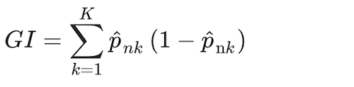
Cross-validation is leveraged again to estimate tuning parameters mtry and B.
Gradient boosting
Gradient boosting relies on weak classifiers that build on each other to produce an ensemble classifier with a lower predictive error (Kuhn and Johnson 2013). Based on Friedman (2001), the approach initializes a tree to fko(X) = 0, k = 1,…, K. Then, it iterates z = 1,…,Z times to generate trees, fkz(X), that build on each other at every z step, estimating the probability of an observation belonging to a class:
(9)
This ratio is taken to ensure that probabilities for all classes add up to one. f(X) defines a tree with a constant value for each terminal node. To estimate the parameters of fk(x) and fh(x), the algorithm uses the following deviance loss function:
(10)
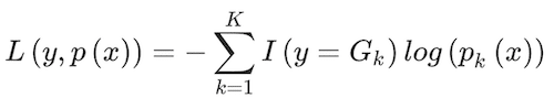
where I(y = Gk) is an indicator conditional function that takes a unit value if the classifier,Gk, holds and zero if it does not. The classifier assigns classes based on what class k gets the greatest pk(X) value. An interesting aspect of gradient boosting is that during each iteration, z, the error is estimated as rikz = Yik-pk(Xi), i = 1,..,N. The value of Yik takes a unit value if it belongs to class k, and zero otherwise. Then, a regression tree using the Xifeatures is fit to the errors rikz, giving terminal regions Rvkz, with v = 1,…Vm terminal nodes. Rvkz is the set of X values that define each terminal node. From here, Friedman (2001) computes:
(11)
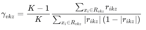
This parameter is used to update the fk(X) of the z iteration, such as
(12)
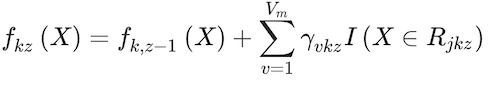
One can think of it as the final gradient boost tree solution.
Four tuning parameters are used in this process: number of boosting iterations, Z, maximum weak learner tree depth, d, shrinkage, or speed of learning, γ and minimum terminal node sample size, u. The tuning parameters estimated via cross-validation are Z, d, s, and u.
Neural Networks
Neural networks are a multi-stage classification (in our case) approach. The relationship between the response and predictor features in the data is intermediated by features engineered by the approach, called hidden units, H. A hidden unit in a single-layer neural network can be described as (Hastie et al. 2009)
(13)
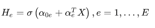
where e = 1,…, E is the number of hidden units in the hidden layer, and σ(X) is a function of the linear component that allows for non-linearities. Then, a linear combination of the engineered features, Tk, is generated for each response variable class:
(14)
A final transformation step estimates the response function. In a multinomial case like the one in this paper, the function is akin to the multinomial logit, here called a softmax function (Bridle 1990), identical to the one seen in the multinomial model above in Eq. (4):
(15)
In addition, following the same algorithm as in the one used in the multinomial logit model, the objective function to be minimized yielding estimates for all parameters (α0m, αm, β0k and βk) is a deviance loss function:
(16)
And the corresponding classifier is G(X) = argmaxk fk(X). Similar to the one used in the learning multinomial logit model, the loss function, in this case, allows for regularization, in the form of a weight decay, λ, that penalises their inclusion of additional parameters (ϴ ∈ {α0m, αm, β0k and βk}) in the model, thus reducing the chance for overfitting
(17)
Cross-validation is used to zero into the two tuning parameters involved in the algorithm, H and λ.
Support vector machines
Support vector machines (SVM) are an extension of maximal margin classifiers and support vector classifiers to accommodate non-linear separation boundaries, also expanding the feature space beyond a two-class setting, using kernels. Kernels, in this context, are inner product functions of predictor features, often represented as K(x,x’) = 〈 xi,xi’〉, capturing the similarity of two observations. Kernels facilitate a computational approach that allows for the inclusion of large numbers of features, most of them engineered.
This form of hinge functions, h(X), can be characterized by nonlinearities often in the form of polynomials, radial and neural network functions. The model becomes:
(18)
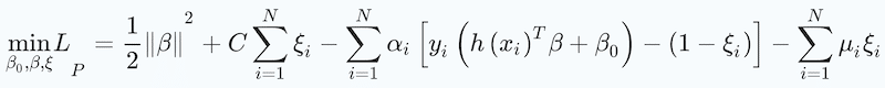
The goal is to find parameter values that maximize the margin, π, which in SVM parlance is the distance between the classification separation boundary and the closest data point. This can be captured as a constrained optimisation of the form:
(19)
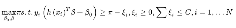
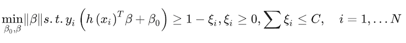
where ξ is a slack factor to allow some error in the classification preventing overfitting and C is an arbitrary constant. This optimisation problem can be turned into a more tractable convex optimisation expression (Hastie et al. 2009)
(20)
It can be taken a step further and turn the expression into
(21)
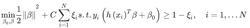
The arbitrary constant C is treated as a tuning parameter. The constrained optimisation can be solved using a Lagrangian method.
(22)
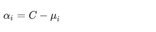
where αi and μ are Lagrangian multipliers. By setting the first derivatives to zero, analytic expressions of the parameters are generated:
(23)
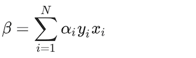
(24)
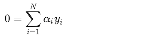
(25)
The approach then substitutes these first-order solutions into the Lagrangian above, to get the optimization for the Lagrangian dual objective function:
(26)
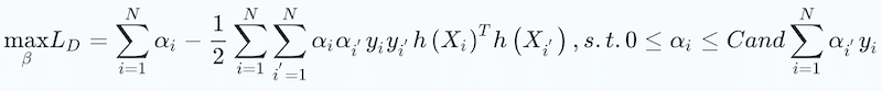
leading to
(27)
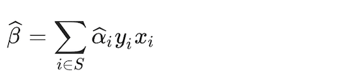
Where S is the collection of indices for which α is equal to zero. α is different from zero for only X values in the training set that are closest to the boundary and are predicted with the least amount of certainty. This reduces the feature space for which to estimate parameters more manageable from a computational standpoint.
Ensemble learning
Ensemble learning is becoming a widely used approach in machine learning (Bajari et al. 2015; Sagi and Rokach 2018). It can take a range of forms but at its core, it is built by combining a collection of underlying models. Some of the machine-learning models applied in this paper are themselves ensemble models, like random forests and gradient boosting.
That is, their final estimate is built from weaker models developed during the estimation process. For the ensemble learning model, here we have used an approach similar to random forests. It estimates the predictions of all machine-learning models on the test observations and applies a majority vote rule approach.
When ties occur, the best-performing model is used for the final prediction.
Results
The objective is to provide a comparison point as to how machine-learning techniques stack up in their ability to predict consumer SKU choices relative to each other and a more traditional statistical technique. While classification models produce both continuous probability estimates and the associated predicted class, the focus is typically the latter.
That makes sense since it tends to be the observable event. As mentioned earlier, the performance of the classification forecast is done out-of-sample, rather than the in-sample. There are several metrics used to determine class forecast performance on test observations. We rely on three commonly used ones including Accuracy (percentage of observations correctly classified), Kappa (similar to Accuracy but it removes the probability that an accurate prediction occurs by chance), and Sensitivity (proportion of observations of class k predicted correctly).
Their values are estimated against a test dataset, instead of the training dataset. Following machine learning’s modelling emphasis on predictive ability rather than interpretation of model parameters, just tuning parameters for each model are reported. Tuning parameters for the seven models are captured in Table 5, while Table 6 contains sensitivities by approach and Table 7 summarises Accuracy and Kappa values by approach.
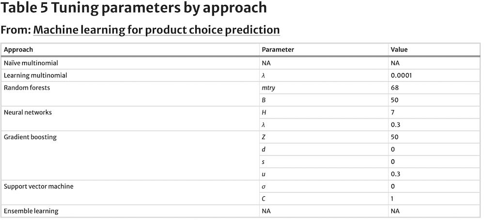
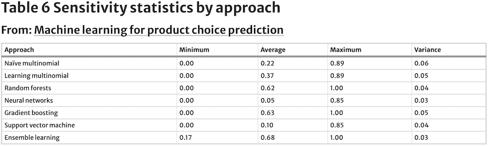
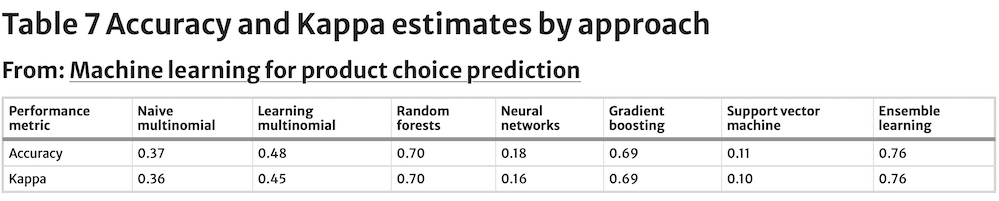
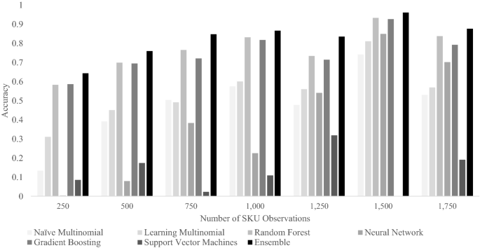
The naïve multinomial logit model is used as the benchmark to evaluate the performance of subsequent machine learning models. It does not have any tuning parameters by design and thus does not have any records in Table 5. Sensitivity ranges from 0.00 to 0.89, with an average value of 0.22, while Accuracy is 0.37. However, we can see in Fig. 1 that prediction Accuracy for this model improves significantly as SKU observations increase.
Kappa is equal to 0.36, coming close to the Accuracy estimate. The closeness between these two numbers is likely a result of the large number of classes being predicted. With as many classes as the ones included in this analysis (149), the likelihood of an accurate prediction being the result of chance becomes small. Thus, the closeness between Accuracy and Kappa.
This is further validated by the fact that we see the same dynamic in results for all approaches presented below. These performance statistics portray our naïve multinomial model as relatively poor at predicting the next SKU purchase by a panelist. However, this low performance should not be surprising, since the model attempts to estimate the next purchase choice by each panelist (out of 3,404) at the SKU level (out of 142), which is a relatively demanding forecasting task.
The learning multinomial logit model’s optimal decay tuning parameter, λ, equals 0.0001, which is a relatively low penalisation. Sensitivity estimates for the SKUs being predicted have a similar range to that observed for the naïve multinomial logit model, with only a slightly greater mean. Accuracy and Kappa for this model also show moderate improvement relative to the benchmark.
Accuracy’s trend improves for SKUs with a larger number of observations, as was the case for the naïve multinomial logit model (Fig. 1). Based on these results, we can conclude that the learning multinomial model performs better than the naïve multinomial model, overall. The improvement in performance by the learning multinomial logit model is a result of just applying data preprocessing and regularisation.
The random forest model selected the tunning parameter mtry to be 68 and B equal to 50. Sensitivity estimates for the SKUs being forecast show a sizable relative improvement vs. the naïve multinomial logit model, and even its learning counterpart. The same can be said about Accuracy and Kappa values. Accuracy is relatively strong for even the lower range of class observations (Fig. 1), but as shown for the prior approaches, it also benefits from a greater number of observations.
The neural network model’s optimal tunning parameters are H = 7 hidden layers and λ = 0.3 decay (Table 6). Accuracy and Kappa are markedly worse than the performance of the naïve multinomial logit model. Also, the range of sensitivities is only slightly narrower but lower on average. This approach shows the weakest performance at the lower range of class observations, with sizable improvements as observations grow (Fig. 1), however. The neural network model thus shows the greatest need for observations to perform well, as far as this dataset is concerned.
The gradient boosting model has four tuning parameters with optimal levels estimated at Z = 50, d = 0, s = 0 and u = 0.3 (Table 5). Accuracy and Kappa resulting from the application of gradient boosting are relatively high, just shy of the values reached by the random forest model, and better than for the benchmark naïve multinomial logit model. Sensitivity is on average also greater than for even the random forest. Accuracy shows relatively robust levels even with few observations (Fig. 1), while still benefiting from greater number of observations.
The support vector machine has two tuning parameters σ and C. Their optimal values are estimated to be σ = 0 and C = 1 (Table 5). The Accuracy and Kappa levels for the SVM model are the lowest of all tested approaches, including the naïve multinomial logit benchmark model, while sensitivity is only slightly better than for the worst performer, the neural network model.
Performance is volatile across the entire range of SKU observations (Fig. 1), without consistent improvements as the number of observations grows. SVM proves to be the weakest and least stable approach for the dataset used. It is worth noting that at 1,500 observations per SKU (Fig. 1), the SVM approach failed to converge, stressing further its relatively unstable behaviour for this dataset.
The ensemble model has no tuning parameters since it is a simple majority vote algorithm. Its range of sensitivities across predicted SKUs is the narrowest and highest on average of all models evaluated. Its superior performance is also reflected by the highest Accuracy and Kappa levels: Accuracy is six percentage points better than the next best model’s (the random forest model). Furthermore, Fig. 1 shows that the ensemble model’s SKU choice prediction outperforms consistently every other model at any number of SKU observations predictions.
Discussion
Machine learning is bringing a great deal of due diligence to our analyses in marketing research. Its focus is largely directed towards improved model predictive performance. Particularly, it is doing so by turning researchers to evaluate multiple forms of a conceptual model, and different alternative techniques to estimating parameters in one single swoop.
Systematisation of alternative approach testing is done with computationally intensive automated algorithms based on tuning parameters and cross-validation. This is a move away from parametric and towards non-parametric methods that do not make explicit assumptions about the functional form of f(X). Non-parametric methods, however, often have higher observational requirements and come at also higher computational costs. Machine learning also increases the likelihood that a model will perform well in a new environment, by splitting observations between training and test datasets. This emphasis is of particular importance to applied research in the commercial fields of marketing, reducing risk for decision-makers.
We compare a naïve multinomial logit product purchase predictive model against six other alternatives: learning multinomial logit, random forests, neural networks, gradient boosting, support vector machines and an ensemble learning algorithm. The results show that random forest and gradient boosting, in that order, perform best among the six single-model approaches (excluding the ensemble model). However, some machine-learning approaches, namely neural networks and support vector machines, resulted in weaker predictive performance.
Both neural network and support vector machine approaches perform worse than even the naïve multinomial logit benchmark model, on average. However, neural network’s relative performance improves significantly with greater observations, surpassing naïve multinomial logit model’s performance at the higher end of observations (Fig. 1). On the other hand, support vector machine’s performance remains low and somewhat volatile across the spectrum of observations (Fig. 1). That is likely a result of the fact that support vector machines is perhaps the most data demanding of all methods tested in this paper, given its reliance on large number of kernels.
An important finding is that the ensemble learning algorithm, which combines predictions, from all the other six models, displays the best predictive performance, six percentage points above the next best approach. This is a result of ensemble learning’s ability to increase predictive accuracy for SKU classes that prove to be difficult to predict by single models.
Conventional wisdom would make us believe that the approach of choice should be to rely on the best-performing single model. Thus, marketing researchers may need to consider not only testing a wide range of machine-learning models to answer specific questions but also taking one step further to generate ensemble solutions as a potential best-in-class approach to generate robust answers in any observational conditions.
The results resonate with findings in similar studies. For example, Bajari et al. (2015) demonstrated that machine learning methods led to superior predictive accuracy relative to the more traditional linear regression or logit models when applied to aggregate demand data. Further, they also found that an ensemble model in the form of a linear combination of the underlying models can improve fit even further, as it is also shown in this paper.
The focus of their work was explaining longitudinal continuous aggregated salty-snacks demand at the store level, rather than predicting individual consumer choice events. This is evidence of the robustness of machine learning across categories and aggregation levels. Some studies point to traditional choice models, like the multinomial logit model used as a benchmark in this paper, as superior to machine learning. Feldman et al. (2022) find that gradient boosting underperforms relative to a traditional multinomial logit model challenger.
They make a side-by-side comparison between the two approaches for two of Alibaba’s marketplaces (Tmall and Taobao), using a randomised field experiment. Specifically, they expose two randomised sets of consumers coming to their websites to product recommendations generated by one of the two models: One set of consumers were exposed to product recommendations from the gradient boosting model and another set of consumers to recommendations from the multinomial logit model.

They then compare the revenue generated per customer visit between the two cells. The results showed a 28% lift in revenue per customer when the recommendations were driven by the multinomial logit model, relative to when gradient boosting was making the recommendations. This finding is a lesson that suggests that we should not always take it as a given that machine-learning techniques are superior. Instead, multiple comparisons should be made against out-of-sample or test datasets.
Even better, the comparisons should be made by applying randomised field experiments, such as Feldman et al. (2022) do. The benefit of this approach is threefold: (1) we can feel confident of the causality behind the results, (2) the model performance comparison is done in a realistic setting that considers operational elements, marketplace dynamics and consumer behaviour, and (3) it is measured against business outcomes rather than statistical measures like accuracy.
Both researchers and practitioners will find value in the flexibility, ease of use, and scalability of machine learning methods for a wide variety of marketing research problems, not just product purchase prediction. Machine learning may have already advanced more amongst practitioners in the marketing research space. This could in part be because it focuses on prediction vs. explanation and validation of theoretical constructs of consumer behaviour.
Marketer incentives may skew more towards getting it right, than understanding the underlying dynamics of consumer choice processes. As a result, the implications of continued improvements in consumer product choice predictions with machine learning loom large for the industry. Both consumers and suppliers, in the form of either manufacturers and/or retailers, can benefit from improvements to consumer product choice prediction.
By applying machine-learning techniques uncertainty of future demand can be reduced, according to the results presented here. This can improve supply chain efficiencies on both the manufacturer and retailer sides significantly—which is an area that continuously tries to find ways to smooth operations and reduce waste. Better forecasts of consumer choice can help manufacturing investment allocations and assortment optimisations. Inventory of idle product costs and penalties incurred by manufacturers for not meeting supply needs by the retailer will be reduced. More significantly it can ensure the relevancy of products presented to the individual consumer, thereby increasing the ROI of marketing and overall CLV to your business, especially when adopted via communication.
Another area improved predictions will impact is a decline in opportunity costs from not having appropriate products ready to meet consumer choices. Consumers unable to find their preferred choice will result in lower levels of satisfaction, and therefore greater churn. Significantly it also results in greater levels of goods being returned, whereas the opposite is true when adopted. Thus, a direct effect of better planning resulting from improved consumer choice predictions will then prevent loyalty erosion on brand and retailer. Academia’s mission, on the other hand, tends to be more focused on the validation of consumer behaviour theories.
It is often argued that traditional methods are better at uncovering the whys behind observed consumer behaviour, while machine learning approaches are better at predicting it. Traditional models are relatively easier to interpret, while machine learning models tend to be more convoluted and difficult to wrap one’s head around. Conventional wisdom may be worth being challenged in future research, though.
There is room to investigate whether machine learning models can yield greater understanding and new hypotheses about consumer behaviour than traditional models. They could do so by leveraging these models in simulation runs under alternative scenarios. The findings could then be confirmed with the application of designs of experiments to truly establish causality. Comparing the learnings of this two-step approach (machine learning-based simulations first, followed by the design of experiments) relative to those from traditional statistical modelling may be worth considering.
Conclusion
It is concluded based on the analysis presented that machine-learning techniques are superior to a traditional approach in predicting consumer product choices, but their performance can vary depending on the approach, and presumably the dataset. In addition to their intrinsic inherent strengths, machine learning techniques consistently follow a series of steps that make them formidable relative to traditional statistical approaches.
These steps include data preprocessing, feature engineering, data splitting between training and test sets, cross-validation, and use of tuning parameters (Kuhn and Johnson 2013). The result of such a painstaking process is more flexible relationships between predictor and predicted features and less over-fitting. The net benefit of such due diligence is better out-of-sample predictions.
A salient aspect of the findings in this paper is that ensemble models that rely on both machine learning and traditional modelling approaches are particularly robust. Best practices in both academic and applied marketing analytics should involve the implementation of multiple modelling approaches, including traditional and machine learning techniques, to analyse every individual study.
This set of multiple diverse models should then be leveraged to generate an ensemble model. This meta-modelling technique is likely to be the most robust, as shown by this and similar papers (Bajari et al. 2015). There is room for further research when it comes to the development and performance of ensemble models in the marketing analytics space.
There are a variety of ways to build this type of models-of-models: combination methods, diversity, ensemble pruning, boosting, clustering, and bagging are just a few of them. Thus, identifying which methods work best for marketing and consumer analytics is a fertile ground for future research.
The chain reaction unleashed by enhanced predictions has two large implications: one for consumers and another for the supply chain stakeholders including manufacturers, distributors, and retailers. Better predictions of future consumer behaviour will anticipate supply needs. With that foresight, meeting those supply needs will then result in fewer out-of-stock messages being encountered by consumers looking for their preferred products.
Fewer out-of-stocks will likely translate into a build-up of consumer satisfaction levels. This buttressing of satisfaction on the part of consumers will likely result in improved loyalty for products, manufacturers, and retailers. A final consequence of this sequential domino reaction started with improved predictions of consumer preferences is that the loyalty increase will help supply chain stakeholders, including manufacturers and retailers, generate better business results.
Although outside of the scope of this paper, an area that may be worth challenging is the maxim that machine learning models are catered for prediction, while traditional statistical models are better at testing hypotheses. If it is established that machine learning models can predict consumer behaviour better, it stands to reason that they should be able to test hypotheses better too.
The way to test hypotheses may require simulations of conditions we are interested in, based on more complex single or ensemble models that may not have theoretical underpinnings. This is a departure from traditional parametric hypothesis testing, but necessary in a world where complex dynamics are recognised (often beyond our ability to understand) and captured. In any case, one can also argue that for true causal hypothesis testing, executions of experimental designs may be needed rather than stopping at just observational data-driven traditional or machine-learning model-generated results.
References
- Bajari, P., D. Nekipelov, S.P. Ryan, and M. Yang. 2015. Machine Learning Methods for Demand Estimation. American Economic Review: Papers & Proceedings 105 (5): 481–485.
Citation: Martínez-Garmendia, J. Machine learning for product choice prediction. J Market Anal(2023).