
Granular computing has been more of a theoretical perspective than a coherent set of methods or principles. As a theoretical perspective, it encourages an approach to data that recognizes and exploits the knowledge present in data at various levels of resolution or scales.
In this sense, it encompasses all methods which provide flexibility and adaptability in the resolution at which knowledge or information is extracted and represented.
As mentioned above, granular computing is not an algorithm or process; there is no particular method that is called “granular computing”. It is rather an approach to looking at data that recognises how different and interesting regularities in the data can appear at different levels of granularity.
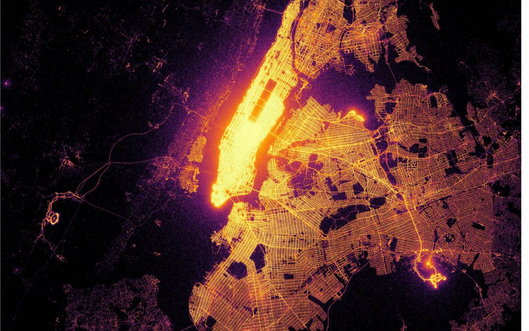
On a low-resolution satellite image, for example, one might notice interesting cloud patterns representing cyclones or other large-scale weather phenomena, while in a higher-resolution image, one misses these large-scale atmospheric phenomena but instead notices smaller-scale phenomena, such as the interesting pattern that is the streets of Manhattan.
The same is generally true of all data: At different resolutions or granularities, different features and relationships emerge. The aim of granular computing is ultimately simply to try to take advantage of this fact in designing more effective machine-learning and reasoning systems.
Several types of granularity are often encountered in data mining and machine learning, and we review them below:
Value granulation (discretisation/quantisation)
One type of granulation is the quantisation of variables. It is very common that in data mining or machine-learning applications, the resolution of variables needs to be decreased to extract meaningful regularities.
An example of this would be a variable such as “outside temperature” (temp), which, in a given application, might be recorded to several decimal places of precision (depending on the sensing apparatus).
However, for purposes of extracting relationships between “outside temperature” and, say, “number of health-club applications” (club), it will generally be advantageous to quantise “outside temperature” into a smaller number of intervals.
Motivations
There are several interrelated reasons for granulating variables in this fashion:
- Based on prior domain knowledge, there is no expectation that minute temperature variations (e.g., the difference between 80–80.7 °F (26.7–27.1 °C)) could have an influence on behaviour driving the number of health club applications.
For this reason, any “regularity” that our learning algorithms might detect at this level of resolution would have to be spurious, as an artefact of overfitting.
By coarsening the temperature variable into intervals the difference between which we do anticipate (based on prior domain knowledge) might influence several health club applications, we eliminate the possibility of detecting these spurious patterns. Thus, in this case, reducing resolution is a method of controlling overfitting. - By reducing the number of intervals in the temperature variable (i.e., increasing its grain size), we increase the amount of sample data indexed by each interval designation.
Then, by coarsening the variable, we increase sample sizes and achieve better statistical estimation. In this sense, increasing granularity provides an antidote to the so-called curse of dimensionality, which relates to the exponential decrease in statistical power with an increase in the number of dimensions or variable cardinality. - For example, a simple learner or pattern recognition system may seek to extract regularities satisfying a conditional probability threshold such as p(Y=yj|X=xi)≥α. In the special case where α=1, this recognition system is essentially detecting the logical implication of the form X=xi→Y=yj or, in other words, “if X=xi, then Y=yj“.
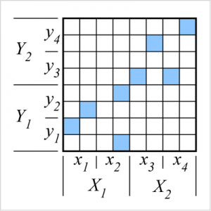
The system’s ability to recognise such implications (or, in general, conditional probabilities exceeding a threshold) is partially contingent on the resolution with which the system analyses the variables. As an example of this last point, consider the feature space shown to the right. The variables may each be regarded at two different resolutions.
Variable X may be regarded at a high (quaternary) resolution wherein it takes on the four values {x1,x2,x3,x4} or at a lower (binary) resolution wherein it takes on the two values {X1, X2}. Similarly, variable Y may be regarded at a high (quaternary) resolution or at a lower (binary) resolution, where it takes on the values {y1,y2,y3,y4} or {Y1, Y2}, respectively.
It will be noted that at the high resolution, there are no detectable implications of the form X=xi→Y=yj since every xi is associated with more than one yj, and thus, for all xi, p(Y=yj|X=xi)<1. However, at the low (binary) variable resolution, two bilateral implications become detectable: X=X1↔Y=Y1 and X=X2↔Y=Y2, since every X1 occurs iff Y1 and X2 occurs iff Y2.
Therefore, a pattern recognition system scanning for implications of this kind would find them at the binary variable resolution but would fail to find them at the higher quaternary variable resolution. Issues and methods. It is not feasible to exhaustively test all possible discretisation resolutions on all variables to see which combination of resolutions yields interesting or significant results.
Instead, the feature space must be preprocessed (often by an entropy analysis of some kind) so that some guidance can be given as to how the discretisation process should proceed. Moreover, one cannot generally achieve good results by naively analysing and discretising each variable independently, since this may obliterate the very interactions that we had hoped to discover.
Variable granulation (clustering/aggregation/transformation)
Variable granulation is a term that could describe a variety of techniques, most of which are aimed at reducing dimensionality, redundancy, and storage requirements. We briefly describe some of the ideas here, and present pointers to the literature.
Variable transformation
Several classical methods, such as principal component analysis, multidimensional scaling, factor analysis, and structural equation modelling, and their relatives, fall under the genus of “variable transformation.” Also in this category are more modern areas of study such as dimensionality reduction, projection pursuit, and independent component analysis.
The common goal of these methods, in general, is to find a representation of the data in terms of new variables, which are a linear or nonlinear transformation of the original variables, and in which important statistical relationships emerge.
The resulting variable sets are almost always smaller than the original variable set, and hence these methods can be loosely said to impose a granulation on the feature space. These dimensionality reduction methods are all reviewed in the standard texts, such as Duda, Hart & Stork (2001), Witten & Frank (2005), and Hastie, Tibshirani & Friedman (2001).
Variable aggregation
A different class of variable granulation methods derive more from data clustering methodologies than from the linear systems theory informing the above methods.
It was noted fairly early that one may consider “clustering” related variables in just the same way that one considers clustering-related data. In data clustering, one identifies a group of similar entities (using a measure of “similarity” suitable to the domain), and then in some sense replaces those entities with a prototype of some kind.
The prototype may be the simple average of the data in the identified cluster or some other representative measure. But the key idea is that in subsequent operations, we may be able to use the single prototype for the data cluster (along with perhaps a statistical model describing how exemplars are derived from the prototype) to stand in for the much larger set of exemplars.
These prototypes generally such as to capture most of the information of interest concerning the entities. - Independent of prior domain knowledge, it is often the case that meaningful regularities (i.e., which can be detected by a given learning methodology, representational language, etc.) may exist at one level of resolution and not at another.
For example, a simple learner or pattern recognition system may seek to extract regularities satisfying a conditional probability threshold such as p(Y=yj|X=xi)≥α. In the special case where α=1, this recognition system is essentially detecting the logical implication of the form X=xi→Y=yj or, in other words, “if X=xi, then Y=yj“.
The system’s ability to recognize such implications (or, in general, conditional probabilities exceeding a threshold) is partially contingent on the resolution with which the system analyzes the variables.
As an example of this last point, consider the feature space shown to the right. The variables may each be regarded at two different resolutions.
Variable X may be regarded at a high (quaternary) resolution wherein it takes on the four values {x1,x2,x3,x4} or at a lower (binary) resolution wherein it takes on the two values {X1, X2}.
Similarly, variable Y may be regarded at a high (quaternary) resolution or at a lower (binary) resolution, where it takes on the values {y1,y2,y3,y4} or {Y1, Y2}, respectively. It will be noted that at the high resolution, there are no detectable implications of the form X=xi→Y=yj since every xi is associated with more than one yj, and thus, for all xi, p(Y=yj|X=xi)<1.
However, at the low (binary) variable resolution, two bilateral implications become detectable: X=X1↔Y=Y1 and X=X2↔Y=Y2, since every X1 occurs iff Y1 and X2 occurs iff Y2.
Thus, a pattern recognition system scanning for implications of this kind would find them at the binary variable resolution but would fail to find them at the higher quaternary variable resolution.
Issues and methods
It is not feasible to exhaustively test all possible discretization resolutions on all variables to see which combination of resolutions yields interesting or significant results. Instead, the feature space must be preprocessed (often by an entropy analysis of some kind) so that some guidance can be given as to how the discretisation process should proceed.
Moreover, one cannot generally achieve good results by naively analysing and discretising each variable independently, since this may obliterate the very interactions that we had hoped to discover.
Variable granulation (clustering/aggregation/transformation)
Variable granulation is a term that could describe a variety of techniques, most of which are aimed at reducing dimensionality, redundancy, and storage requirements. We briefly describe some of the ideas here, and present pointers to the literature.
Variable transformation
Several classical methods, such as principal component analysis, multidimensional scaling, factor analysis, and structural equation modelling, and their relatives, fall under the genus of “variable transformation.”
Also in this category are more modern areas of study such as dimensionality reduction, projection pursuit, and independent component analysis. The common goal of these methods, in general, is to find a representation of the data in terms of new variables, which are a linear or nonlinear transformation of the original variables, and in which important statistical relationships emerge.
The resulting variable sets are almost always smaller than the original variable set, and hence these methods can be loosely said to impose a granulation on the feature space. These dimensionality reduction methods are all reviewed in the standard texts, such as Duda, Hart & Stork (2001), Witten & Frank (2005), and Hastie, Tibshirani & Friedman (2001).
Variable aggregation
A different class of variable granulation methods derive more from data clustering methodologies than from the linear systems theory informing the above methods. It was noted fairly early that one may consider “clustering” related variables in just the same way that one considers clustering-related data.
In data clustering, one identifies a group of similar entities (using a measure of “similarity” suitable to the domain), and then in some sense replaces those entities with a prototype of some kind. The prototype may be the simple average of the data in the identified cluster or some other representative measure.
But the key idea is that in subsequent operations, we may be able to use the single prototype for the data cluster (along with perhaps a statistical model describing how exemplars are derived from the prototype) to stand in for the much larger set of exemplars.
These prototypes generally such as to capture most of the information of interest concerning the entities.
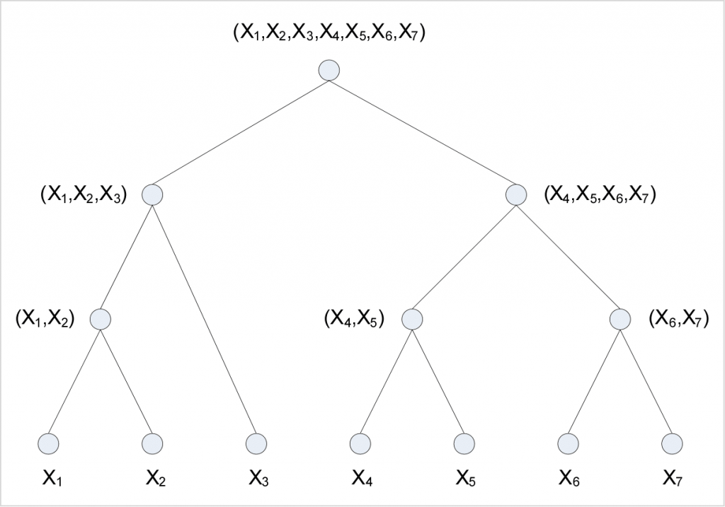
A Watanabe-Kraskov variable agglomeration tree. Variables are agglomerated (or “unitized”) from the bottom-up, with each merge node representing a (constructed) variable having entropy equal to the joint entropy of the agglomerating variables.
Therefore, the agglomeration of two many variables X1 and X2 having individual entropies H(X1) and H(X2) yields a single m2-ary variable X1,2 with entropy H(X1,2)=H(X1, X2).
When X1 and X2 are highly dependent (i.e., redundant) and have large mutual information I(X1; X2), then H(X1,2)≪ H(X1)+H(X2) because H(X1, X2)=H(X1)+H(X2)−I(X1; X2), and this would be considered a parsimonious unitization or aggregation.
Similarly, it is reasonable to ask whether a large set of variables might be aggregated into a smaller set of prototype variables that capture the most salient relationships between the variables.
Although variable clustering methods based on linear correlation have been proposed (Duda, Hart & Stork 2001; Rencher 2002), more powerful methods of variable clustering are based on the mutual information between variables.
Watanabe has shown (Watanabe 1960; Watanabe 1969) that for any set of variables one can construct a polytonic (i.e., n-ary) tree representing a series of variable agglomerations in which the ultimate “total” correlation among the complete variable set is the sum of the “partial” correlations exhibited by each agglomerating subset (see figure).
Watanabe suggests we might seek to partition a system in such a way as to minimize the interdependence between the parts “… as if they were looking for a natural division or a hidden crack.”
One practical approach to building such a tree is to successively choose for agglomeration the two variables (either atomic variables or previously agglomerated variables) which have the highest pairwise mutual information (Kraskov et al. 2003).
The product of each agglomeration is a new (constructed) variable that reflects the local joint distribution of the two agglomerating variables and thus possesses an entropy equal to their joint entropy.
From a procedural standpoint, this agglomeration step involves replacing two columns in the attribute-value table—representing the two agglomerating variables—with a single column that has a unique value for every unique combination of values in the replaced columns (Kraskov et al. 2003).
No information is lost by such an operation; however, it should be noted that if one is exploring the data for inter-variable relationships, it would generally not be desirable to merge redundant variables in this way, since in such a context it is likely to be precisely the redundancy or dependency between variables that are of interest; and once redundant variables are merged, their relationship to one another can no longer be studied.
System granulation (aggregation)
In database systems, aggregations (see e.g. OLAP aggregation and Business intelligence systems) result in transforming original data tables (often called information systems) into tables with different semantics of rows and columns, wherein the rows correspond to the groups (granules) of original tuples and the columns express aggregated information about original values within each of the groups.
Such aggregations are usually based on SQL and its extensions. The resulting granules usually correspond to the groups of original tuples with the same values (or ranges) over some pre-selected original columns.
There are also other approaches wherein the groups are defined based on, e.g., the physical adjacency of rows. For example, Infobright implemented a database engine wherein data was partitioned onto rough rows, each consisting of 64K physically consecutive (or almost consecutive) rows.
Rough rows were automatically labelled with compact information about their values on data columns, often involving multi-column and multi-table relationships. It resulted in a higher layer of granulated information where objects corresponded to rough rows and attributes – to various aspects of rough information. Database operations could be efficiently supported within such a new framework, with access to the original data pieces still available Template: Slezak.
Concept granulation (component analysis)
The origins of the granular computing ideology are to be found in the rough sets and fuzzy sets work of literature. One of the key insights of rough set research—although by no means unique to it—is that, in general, the selection of different sets of features or variables will yield different concept granulations.
Here, as in elementary rough set theory, by “concept” we mean a set of entities that are indistinguishable or indiscernible to the observer (i.e., a simple concept), or a set of entities that are composed of such simple concepts (i.e., a complex concept).
To put it in other words, by projecting a data set (value-attribute system) onto different sets of variables, we recognise alternative sets of equivalence-class “concepts” in the data, and these different sets of concepts will, in general, be conducive to the extraction of different relationships and regularities.
Equivalence class granulation
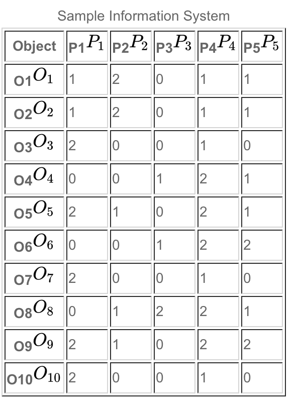
We illustrate with an example. Consider the attribute-value system below:
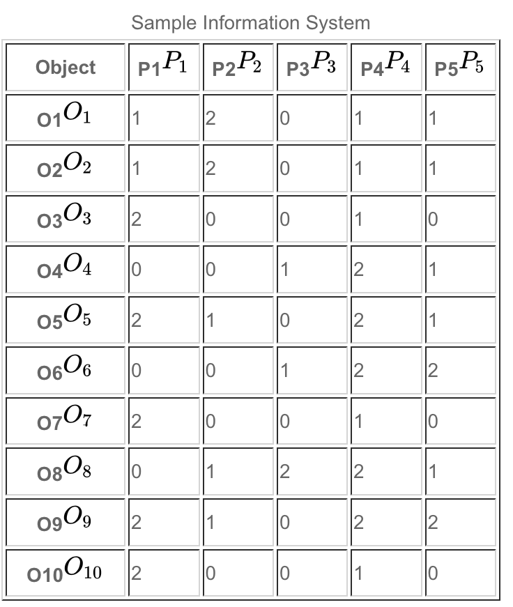
When the full set of attributes P={P1, P2, P3, P4, P5} is considered, we see that we have the following seven equivalence classes or primitive (simple) concepts:{{O1,O2}{O3,O7,O10}{O4}{O5}{O6}{O8}{O9}
Thus, the two objects within the first equivalence class, {O1, O2}, cannot be distinguished from one another based on the available attributes, and the three objects within the second equivalence class, {O3, O7, O10}, cannot be distinguished from one another based on the available attributes.
The remaining five objects are each discernible from all other objects. Now, let us imagine a projection of the attribute value system onto attribute P1 alone, which would represent, for example, the view from an observer which is only capable of detecting this single attribute. Then we obtain the following much coarser equivalence class structure.{{O1,O2}{O3,O5,O7,O9,O10}{O4,O6,O8}
This is in certain regard the same structure as before, but at a lower degree of resolution (larger grain size). Just as in the case of value granulation (discretisation/quantisation), relationships (dependencies) may emerge at one level of granularity that is not present at another.
As an example of this, we can consider the effect of concept granulation on the measure known as attribute dependency (a simpler relative of the mutual information).
To establish this notion of dependency (see also rough sets), let [x]Q={Q1, Q2, Q3,…, QN} represent a particular concept granulation, where each Qi is an equivalence class from the concept structure induced by attribute set Q.
For example, if the attribute set Q consists of attribute P1 alone, as above, then the concept structure [x]Q will be composed of Q1={O1, O2}, Q2={O3, O5, O7, O9, O10}, and Q3={O4, O6, O8}. The dependency of an attribute set Q on another attribute set P, γP(Q), is given

That is, for each equivalence class Qi in [x]Q, we add up the size of its “lower approximation” by the attributes in P, i.e., P_Qi. More simply, this approximation is the number of objects which on the attribute set P can be positively identified as belonging to the target set Qi.
Added across all equivalence classes in [x]Q, the numerator above represents the total number of objects which—based on attribute set P—can be positively categorised according to the classification induced by attributes Q.
The dependency ratio, therefore, expresses the proportion (within the entire universe) of such classifiable objects, in a sense capturing the “synchronisation” of the two concept structures [x]Q and [x]P. The dependency γP(Q) “can be interpreted as a proportion of such objects in the information system for which it suffices to know the values of attributes in P to determine the values of attributes in Q” (Ziarko & Shan 1995).
Having gotten definitions now out of the way, we can make the simple observation that the choice of concept granularity (i.e., choice of attributes) will influence the detected dependencies among attributes. Consider again the attribute value table from above:
Let us consider the dependency of the attribute set Q={P4, P5} on the attribute set P={P2, P3}. That is, we wish to know what proportion of objects can be correctly classified of [x]Q based on knowledge of [x]P. The equivalence classes of [x]Q and of [x]P are shown below.
| [x]Q | [x]P |
|---|---|
| {{O1,O2}{O3,O7,O10}{O4,O5,O8}{O6,O9} | {{O1,O2}{O3,O7,O10}{O4,O6}{O5,O9}{O8} |
The objects that can be definitively categorised according to concept structure [x]Q based on [x]P are those in the set {O1, O2, O3, O7, O8, O10}, and since there are six of these, the dependency of Q on P, γP(Q)=6/10.
This might be considered an interesting dependency in its own right, but perhaps in a particular data mining application, only stronger dependencies are desired.
We might then consider the dependency of the smaller attribute set Q={P4} on the attribute set P={P2, P3}. The move from Q={P4, P5} to Q={P4} induces a coarsening of the class structure [x]Q, as will be seen shortly.
We wish again to know what proportion of objects can be correctly classified into the (now larger) classes of [x]Q based on knowledge of [x]P. The equivalence classes of the new [x]Q and of [x]P are shown below.
| [x]Q | [x]P |
|---|---|
| {{O1,O2,O3,O7,O10}{O4,O5,O6,O8,O9} | {{O1,O2}{O3,O7,O10}{O4,O6}{O5,O9}{O8} |
[x]Q has a coarser granularity than it did earlier. The objects that can now be definitively categorized according to the concept structure [x]Q based on [x]P constitute the complete universe {O1, O2,…, O10}, and thus the dependency of Q on P, γP(Q)=1.
That is, knowledge of membership according to category set [x]P is adequate to determine category membership in [x]Q with complete certainty; In this case, we might say that P→Q. Thus, by coarsening the concept structure, we were able to find a stronger (deterministic) dependency.
However, we also note that the classes induced in [x]Q from the reduction in resolution necessary to obtain this deterministic dependency are now themselves large and few; as a result, the dependency we found, while strong, may be less valuable to us than the weaker dependency found earlier under the higher resolution view of [x]Q.
In general, it is not possible to test all sets of attributes to see which induced concept structures yield the strongest dependencies, and this search must be therefore be guided with some intelligence. Papers which discuss this issue, and others relating to intelligent use of granulation, are those by Y.Y. Yao and Lotfi Zadeh.
Component granulation
Another perspective on concept granulation may be obtained from work on parametric models of categories. In mixture model learning, for example, a set of data is explained as a mixture of distinct Gaussian (or other) distributions. Thus, a large amount of data is “replaced” by a small number of distributions.
The choice of the number of these distributions, and their size, can again be viewed as a problem of concept granulation. In general, a better fit to the data is obtained by a larger number of distributions or parameters, but to extract meaningful patterns, it is necessary to constrain the number of distributions, thus deliberately coarsening the concept resolution.
Finding the “right” concept resolution is a tricky problem for which many methods have been proposed (e.g., AIC, BIC, MDL, etc.), and these are frequently considered under the rubric of “model regularization”.
Different interpretations of granular analysis computing
Granular computing can be conceived as a framework of theories, methodologies, techniques, and tools that make use of information granules in the process of problem-solving. In this sense, granular computing is used as an umbrella term to cover topics that have been studied in various fields in isolation.
By examining all of these existing studies in light of the unified framework of granular computing and extracting their commonalities, it may be possible to develop a general theory for problem-solving.
In a more philosophical sense, granular computing can describe a way of thinking that relies on the human ability to perceive the real world under various levels of granularity (i.e., abstraction) to abstract and consider only those things that serve a specific interest and to switch among different granularities.
By focusing on different levels of granularity, one can obtain different levels of knowledge, as well as a greater understanding of the inherent knowledge structure.
Granular computing is thus essential in human problem solving and hence has a very significant impact on the design and implementation of intelligent systems.
See this crucial software comparison article:
Distinctions between all the top hyper-personalisation software providers (Updated)